Engineering note

LLAMA 1B Optimizing Kernels

Notes on optimizing kernels for Llama 1B

April 7, 2026

llamakernels

Introduction & Motivation

This project explores the design and implementation of a custom LLaMA 1B inference engine, built from the ground up using Apple’s Metal API and tinygrad as a Metal Backend. This implementation focuses on hand-coded GPU kernels to discover some of the optimizations applied by the current compilers such as XLA and tinygrad.

For the written kernels and details about the runner you can see the full project at Llama Runner (Github).

Metal Backend

For the interaction between the runner and the MacBook GPU, all that was needed was a compiler for the Metal kernels that make up the Llama layers + a memory allocator to handle the activations and weight buffers. Tinygrad already handles all of these for their custom Metal backend, so I took most of the utilities from there.

I used metal and metallib to compile and link kernels into a single MTLbinary. Then the MetalProgramtinygrad class was used to manage the GPU command queue and handle kernel execution.

Memory management utilized tinygrad’s MetalAllocator. To minimize allocations, I used the _copyin method to load weights for each successive layer into the same buffer, trying to reuse memory as much as possible across inference.

The tokenizer was copied from tinygrad/examples/llama3.py and the weights were fetched from Llama1B (GGUF) and converted into a dictionary of layer tensors. While all shape transformation such as transposing and flattening were performed in high-level tinygrad, raw memory buffer pointers were accessed via the _buffer()._buf private API to interface with the MetalProgram.

Model Architecture & Shapes

Shapes and Configuration

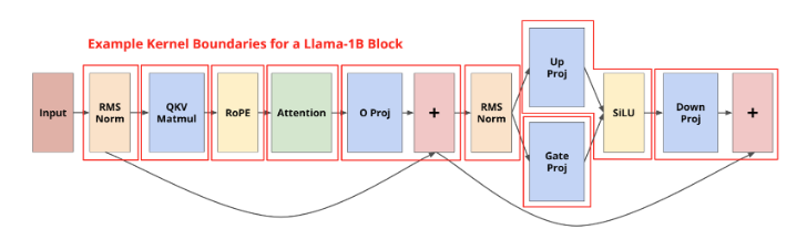
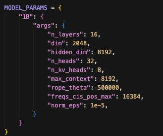
Each transformer block follows the layer structure of Figure 1. This architecture consists of 16 transformer blocks with a hidden dimension ($d_{model}$) of 2048 and an intermediate MLP size of 8192. These dimensions are important for defining launch configurations and hardware-to-data mapping in each one of the hand coded kernels.

While the model weight shapes are static, the activation shapes vary based on the user prompt. We define a fixed processing shape and pad the activations as needed to ensure their dimensions are integer multiples of this configuration.

Decode vs Prefill

For simplicity in this first version, the model is implemented as decode-only. LLM inference typically involves two distinct stages: prefill and decode.

• Prefill: The model computes attention for the entire user prompt (length $T$) and populates the KV cache with $T$ projections. These $T$ projections can be done in parallel, achieving better occupancy of GPU cores (the Metal equivalent of SMs), resulting in higher throughput.
• Decode: The model generates tokens one by one (including the user prompt), calculating $Q$, $K$, and $V$ vectors of shape $(B, T=1, n\_heads \times dim)$. These shapes (especially when running with batch_size=1) do not fully occupy all of the processing cores we have available. Separating these stages optimizes performance but requires writing distinct kernels for each: GEMM (General Matrix-Matrix Multiplication) + prefill attention for one stage and GEMV (General Matrix-Vector Multiplication) + decode attention for the other stage.

Grouped Query Attention (GQA)

Based on the model parameters, this architecture employs Grouped Query Attention (GQA). It features 32 query heads and 8 KV heads, meaning each group of four query heads attends to a single shared KV head. This configuration reduces the KV cache memory by a factor of four, as only 8 heads are appended to the cache during each decoding step, rather than the 32 heads required by standard Multi-Head Attention (MHA).

Custom Kernels

Flash Attention

Flash Attention 2 Flash Attention 2 paper describes attention optimizations designed to achieve significant speedups across both forward and backpropagation passes particularly when sequence length $T > 1$. Because my implementation is currently decode-only, I have adjusted these mappings to accommodate the single-query-token structure.

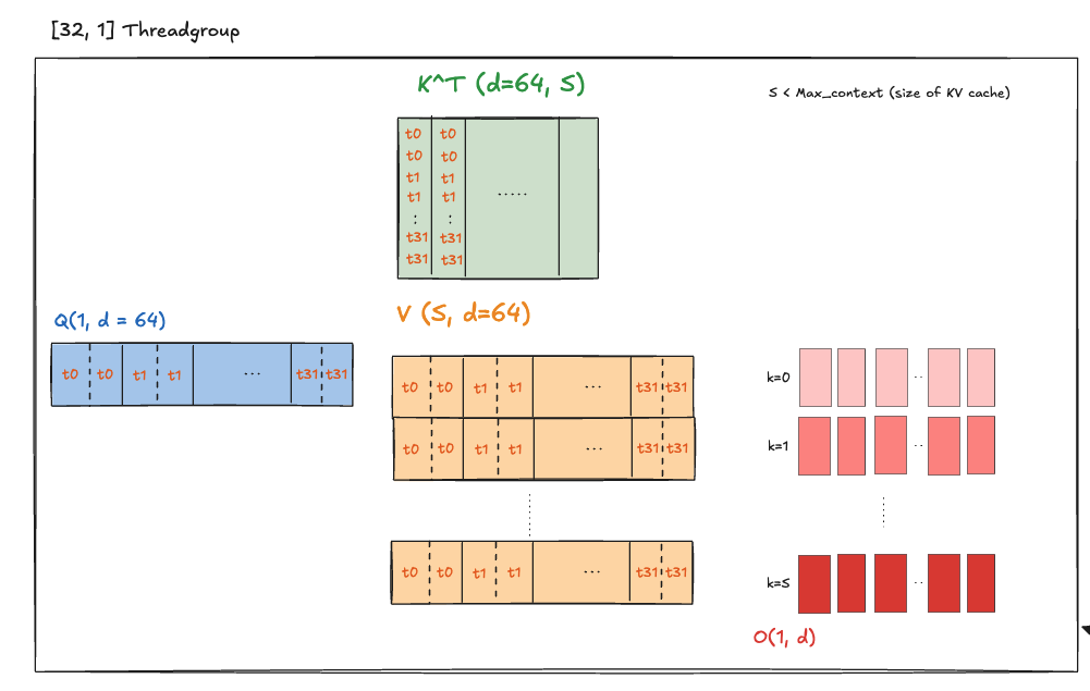
As illustrated in Figure 3, each thread manages 2 lanes of the head dimension ($d$). By launching with threadgroups of 32 (exactly matching a Metal simdgroup), I can cover the entire Query row projection with a single threadgroup.

Since each threadgroup is mapped to a single Query head ($Q$-head) and this LLaMA architecture contains only 32 heads, the execution is limited to a total of 32 threadgroups. This results in significantly low GPU occupancy, as it fails to provide enough concurrent work to saturate the hardware’s available execution units.

In the kernel logic, each thread iterates across the sequence dimension ($S$) where kernel applies the online softmax correction introduced in FA. Because this is a decode-only kernel, causal masking is not required; the single query row being processed attends to the entire KV cache (up to max_context).

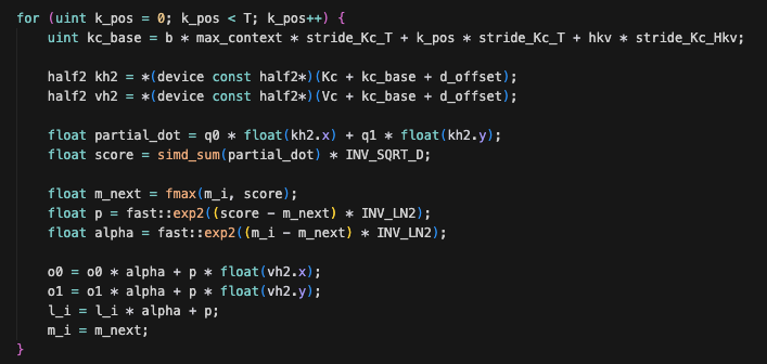
I am still exploring optimizations to improve this implementation. The primary bottleneck is the kernel’s low arithmetic intensity. In a prefill kernel, $K^T$ columns and $V$ rows are reused across multiple token outputs, yielding higher FLOPS per byte loaded. In this decode-only version, however, those values are only used once (for the current decode token).

GEMV

CUTLASS: Fast Linear Algebra In the decode-only series of kernels, the projections and linear layers follow the standard vector-matrix multiplication shape (where $x: [1, K]$ and $W: [K, N]$):

$\mathbf{y} = \mathbf{x} \mathbf{W}$

The kernel I wrote utilizes threadgroups of shape $(32, 4)$, processing the $K$ dimension in tiles of $B_K = 128$. This configuration was determined through autotuning, benchmarking a set of parameters to find the optimal balance between

• Data Reuse: Increasing $B_K$ allows for more significant reuse of loaded elements from $\mathbf{x}$, reducing global memory pressure.
• Occupancy: Lowering $B_K$ increases the total number of threadgroups that can be dispatched, which helps hide latency and improves GPU occupancy.

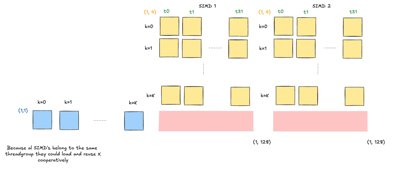
The kernel implements a series of $K$ outer products in blocks of $B_K$ within an inner loop. This structure allows the loaded elements of $\mathbf{x}$ to be reused across $B_K$ rows of $\mathbf{W}$: $\mathbf{y} = \sum_{k=0}^{K-1} x_k \cdot \mathbf{w}_{k, \ast}$

Execution Pipeline:

1. Cooperative Loading: Each threadgroup cooperatively loads $B_K$ elements of $\mathbf{x}$ into threadgroup memory (tg_mem, the Metal equivalent of CUDA shared memory).
2. Vectorized Loads: Each thread performs a vectorized float4 load to fetch four elements across the $N$ dimension. Consequently, each threadgroup handles 512 elements along $N$ ($128$ threads $\times$ $4$ elements).
3. Outer Product Accumulation: The kernel calculates the outer product $x_k \cdot \mathbf{w}_{k, tid:tid+4}$ for $B_K$ iterations, reusing the values of $\mathbf{x}$ stored in tg_mem.
4. Iteration: This cycle (loading into tg_mem followed by $B_K$ outer products) repeats until the entire $K$ dimension is processed.

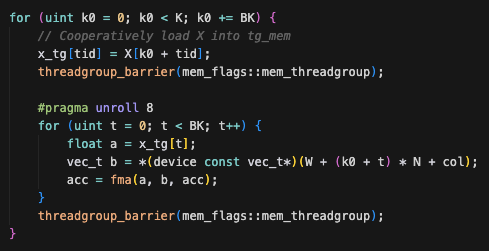
There is a fundamental trade-off when selecting the local_size. Ideally, a single threadgroup would cover the entire $N$ dimension, allowing $\mathbf{x}$ to be loaded only once per $K/B_K$ iteration and reused across the entire row of $\mathbf{W}$.However, hardware constraints limit the amount of available tg_mem per simdgroup. Because the required tg_mem per threadgroup directly impacts the number of active threadgroups that can run in parallel, maximizing reuse often comes at the cost of reduced occupancy.

RMSNorm

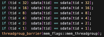
Optimizing Reduction (Mark Harris) In the LLaMA model, the normalization method used is RMSNorm, which requires calculating a normalization factor across the $d$-dimension. To optimize this, I implemented a reduction-style kernel based on Mark Harris’s optimizations.

The first stage of the kernel utilizes vectorized half2 loads to accumulate values into each thread’s local registers. By performing these loads four times per thread, the kernel reduces the $d$-dimension ($d=2048$) down to the launched localsize of 256 threads.

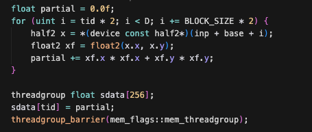
Once the initial 256 partial sums are computed, they are written into threadgroup memory to begin the tree reduction phase. This stage uses sequential addressing. By having threads access indices that are far apart and then narrowing the gap, we avoid bank conflicts—preventing the serialized loads from tg_mem that occur when multiple threads in a SIMDgroup target the same memory bank.

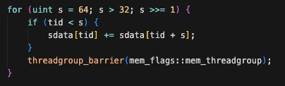
When only 64 partials remain in tg_mem, the tree reduction loop can be unrolled. Once the work is reduced to 32 threads (a single Metal SIMDgroup), the operations become naturally synchronized, alllowing removal of threadgroup barriers.

Kernel Fusion

While the previously described optimizations are performant in an isolated environment, executing 16 transformer blocks results in hundreds of kernel dispatches per forward pass. At this scale, two primary bottlenecks emerge:

• Launch Overhead: Significant time is spent on setup and teardown for each kernel call, during which no useful computation occurs.
• Memory Roundtrips: Each independent kernel must read from and write back to device memory ($RAM$ in Metal’s UMA), creating unnecessary bandwidth pressure as the output of one step becomes the input of the next. To mitigate these issues, I combined the individual operations into three main fused kernels, which keeps data in registers or threadgroup memory as long as possible.

RMSNorm + GEMV

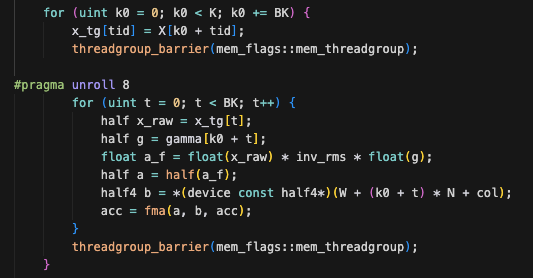
In this fused kernel, the raw activations ($x_{raw}$) are normalized using a previously calculated normalization factor ($inv\_rms$) directly within the GEMV outer product loop. By performing the normalization on-the-fly, we eliminate the need to write the intermediate normalized activations back to global memory.

RMSNorm + 2 GEMV (Up, Gate) + SwiGLU

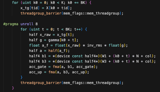
The activations are normalized and then used to calculate two GEMVs simultaneously, the Up and Gate projections. Both projections reuse the same activations already loaded into threadgroup memory (tg_mem). Finally, the SwiGLU activation function is applied to the results of these two projections before a single combined result is written back to device memory.

GEMV (Down) + Residual Add

The final stage of the transformer block fuses the Down projection with the residual connection. After the GEMV calculation is complete, but before the data is committed to global memory, the residual addition is performed in-place.

Performance Analysis (Roofline Model)

To analyze kernel performance effectively, I utilized a profiling model based on device-specific capabilities, specifically theoretical peak FLOPs and memory bandwidth. These metrics form the basis of the Roofline Model, which evaluates hardware limits against the nature of the specific computational problem, defined by its Arithmetic Intensity (AI).

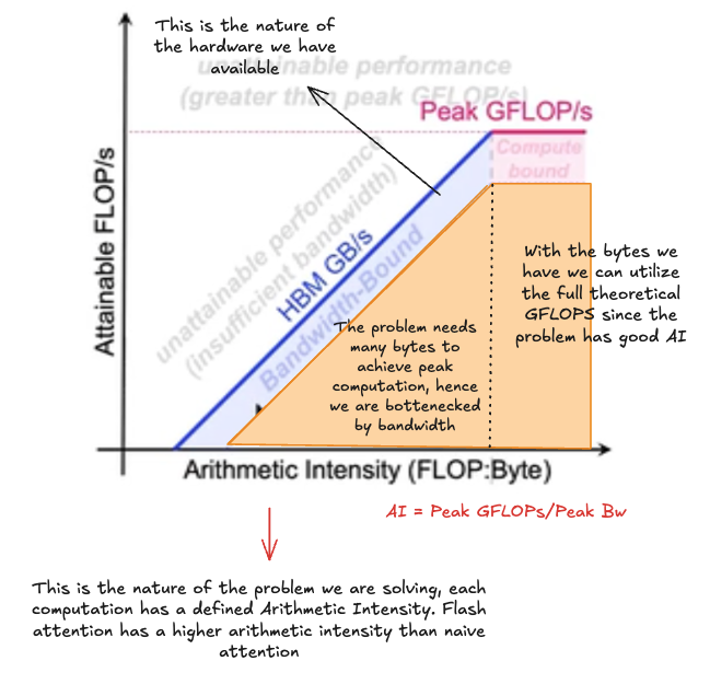
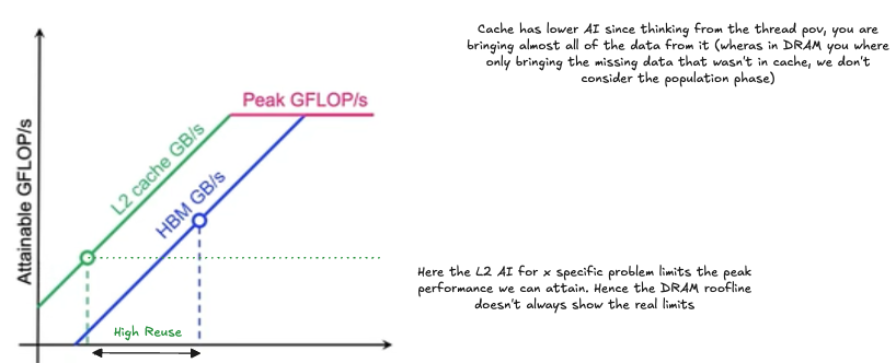
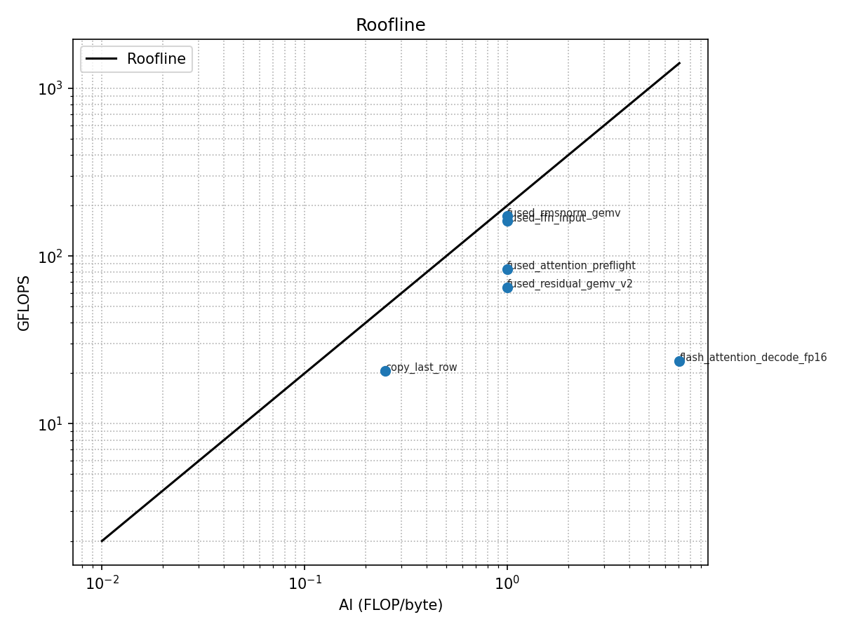
The Roofline Model demonstrates that for a problem with a given arithmetic intensity ($AI = \frac{\text{FLOPs}}{\text{Bytes}}$), performance is governed by two regimes. In the memory-bound region, performance is limited by how fast data can be moved from memory. In the compute-bound region, performance is limited by the hardware’s maximum throughput ($GFLOP/s$). If a kernel falls into the “underperforming” zone (the orange region in Figure 12), it indicates that the implementation is not saturating the available bandwidth or execution units, suggesting room for optimization. Modern GPUs feature a complex memory hierarchy and specialized compute units. Because different layers (L1, L2, and VRAM) have vastly different bandwidths, a kernel has a distinct AI for each level of the hierarchy. Furthermore, specialized units like Tensor Cores (or Apple’s AMX) offer significantly higher theoretical FLOPs than standard execution units. Figure 13 illustrates a scenario where a problem is limited by L2 cache bandwidth, placing it in a region of seemingly “poor performance” when measured only against global memory limits. This could be the explanation of the poor performance of FA decode in Figure 14.

When applied to the LLaMA 1B model (considering the $VRAM$ level of the hierarchy), the profiling shows that the model is strictly memory-bound (Figure 14). For a decode-only model, the primary performance metric is tokens per second ($tok/s$). An upper-bound estimation for attainable speed on a memory-bound device can be expressed as:

$\frac{tok}{s} \approx \frac{\text{Bandwidth}}{\sum \text{Weights}_i}$

This formula represents a theoretical ceiling, as it assumes 100% bandwidth utilization and only accounts for weight loading. In practice, the actual performance will be lower due to the overhead of moving activations and managing the KV cache, which increases in size and complexity as the sequence length grows.

Conclusion

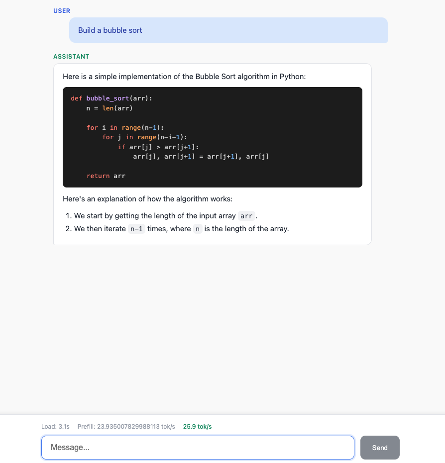
My current implementation of the LLaMA 1B model achieves 26 tokens/s, which is a solid start but remains significantly below the estimated upper bound of ~100 tokens/s supported by the M2 Pro and its 200 GB/s memory bandwidth. This performance gap indicates that while the kernels are functional, the system is not yet fully saturating the hardware, leaving considerable room for optimization.

The next phase of development will focus on the Megakernelconcept, an optimization strategy introduced by HazyResearch. The goal of a Megakernel is to keep weights and activations resident in high-speed, on-chip memory as long as possible. By implementing paged shared memory, the model can drastically reduce the number of expensive global memory ($VRAM$) reads and writes, as well as launch/teardown costs of multiple kernels.

Sources

METAL Spec: https://developer.apple.com/metal/Metal-Shading-Language-Specification.pdf Flash Attention paper: https://arxiv.org/pdf/2205.14135 CUTLASS GEMM: https://developer.nvidia.com/blog/cutlass-linear-algebra-cuda/?utm_source=chatgpt.com Optimizing GEMM (Simon Boehm): https://siboehm.com/articles/22/CUDA-MMM Megakernels: https://hazyresearch.stanford.edu/blog/2025-05-27-no-bubbles Reduction optimizations: https://developer.download.nvidia.com/assets/cuda/files/reduction.pdf Roofline Model: https://developer.nvidia.com/gtc/2020/video/s21565