Engineering note

Inside an LLM Inference Engine: From Request to Response with MTLQwen

What is it like to build an inference engine from scratch, which beats llama.cpp on Qwen 3.5.

September 11, 2026

What is an Inference Engine

A definition I use for inference engines is that they are the orchestration layer of the complete LLM workflow. They handle the memory LLMs need, whether in permanent buffers, such as weights, or “temporary” ones, such as caches. They also handle the compute an LLM performs by orchestrating the execution of all its kernels. Finally, they make it possible to run this workflow for multiple requests concurrently, extracting more performance from these models.

Why I built MTLQwen?

MTLQwen is an inference engine I built specifically for the Qwen 3.5 and 3.8 architecturesThe engine was originally built for Qwen 3.5, but Qwen 3.8 has the exact same architecture, so it works natively with it., focusing on Metal backend for Apple GPUs. It started as a project to learn how inference engines work, but as I went deeper, I realized that specializing it for Qwen and Metal could provide more performance than general purpose inference engines (vLLM or llama.cpp) on this specific model family and hardware. By using Metal specific features and optimizing Qwen’s kernels, MTLQwen ended up outperforming llama.cpp at both batch size 1 and in aggregate throughput, with a further 30% speedup when using DFlash.

Following one batch through MTLQwen

Model Load & Compilation

Before getting into how the engine handles a request, we first have to initialize it. What does initialization mean here? There are three main steps: memory-mapping the model weights, selecting and compiling the kernels needed by each linear layer, and building metadata such as the RoPE tables.

The weights are loaded through mmap, which maps the model file into the process address space and lets the operating system move its pages from SSD into RAM as they are accessed. This avoids loading the entire model at once and causing a large memory spike during initialization. Since we are running on a unified memory architecture, the GPU can then access these weights without requiring a separate copy in discrete GPU memory.

Because the model is quantized, the kernel used by each linear layer depends on both the quantization type and the shape of its weights. The quantization type determines how the weights are packed and dequantized, while the shape determines the tiling and dispatch configuration that works best with it (maximizing occupation). Only the kernel variants required by the model are compiled into Metal pipeline states, which are later bound to command encoders A ComputeCommandEncoder records which PipelineState (an executable kernel) to run, the resource bindings for the buffers it touches, and the dispatch dimensions. Encoders are stored inside a CommandBuffer, which I mostly treat as their submission wrapper, and that buffer is then committed to the GPU CommandQueue. Every GPU operation, including rendering and compute kernels, is ultimately submitted through this CommandQueue. when the kernels are dispatched. Since the same variants are reused across the 32 decoder layers, each pipeline state is built once and then cached.

Finally, we build the metadata needed by these kernels, including the RoPE tables. These tables contain the precomputed rotations for every supported token position, avoiding the need to recalculate the sine and cosine values during each forward pass.

A Request Becomes a Sequence

The engine can receive requests from many kinds of frontends, whether they come from a multi-turn chat, an agentic TUI, or any other interface. The frontend is responsible for applying the model’s chat template and concatenating the conversation’s messages:

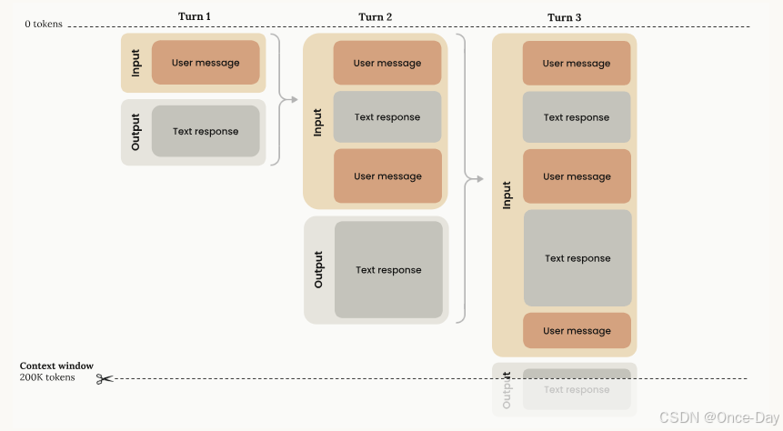
The resulting text is then tokenized, producing the token IDs ready to enter into the inference engine. When the frontend submits a request, represented as an array of token IDs, the engine assigns it to one of eight available slots. These slots determine the maximum number of requests that can be active concurrently.

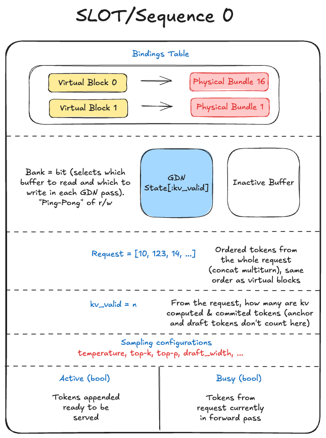
Each slot (also called Sequence in the code) contains the state the engine needs to process its assigned request. Its bindings table maps each part of the request’s KV cache to its location in physical memory, which we will explore in more detail later (Appendix A: Sparse Buffers). A bank bit tells the linear attention kernels which state buffer to read from and which one to write to, with the buffers alternating roles in a ping-pong pattern between forward passes. The request itself is an array of token IDs: it begins with the tokenized prompt and chat template, and each newly sampled token is appended to it. The kv_valid field records how many of those tokens already have valid KV state. During ordinary decoding, the most recently sampled token, also called the anchor token, has not yet passed through the model, so kv_valid = len(request) - 1. During speculative decoding, kv_valid also indicates how many proposed tokens were accepted by the target model and therefore have valid computed state. The busy flag indicates that some of the sequence’s tokens are currently participating in a forward pass, whereas active indicates that the sequence is live and still has work to perform.

Prefix Cache

Most LLM applications combine the user’s message with a system prompt and tool definitions before sending a request to the model. Because this content forms a shared prefix across requests, the engine can compute its state once and reuse it.

The prefix cache stores checkpoints of this state for progressively longer token prefixes. Each checkpoint is identified by a chained hash, allowing the engine to find previously computed state without comparing entire token sequences.

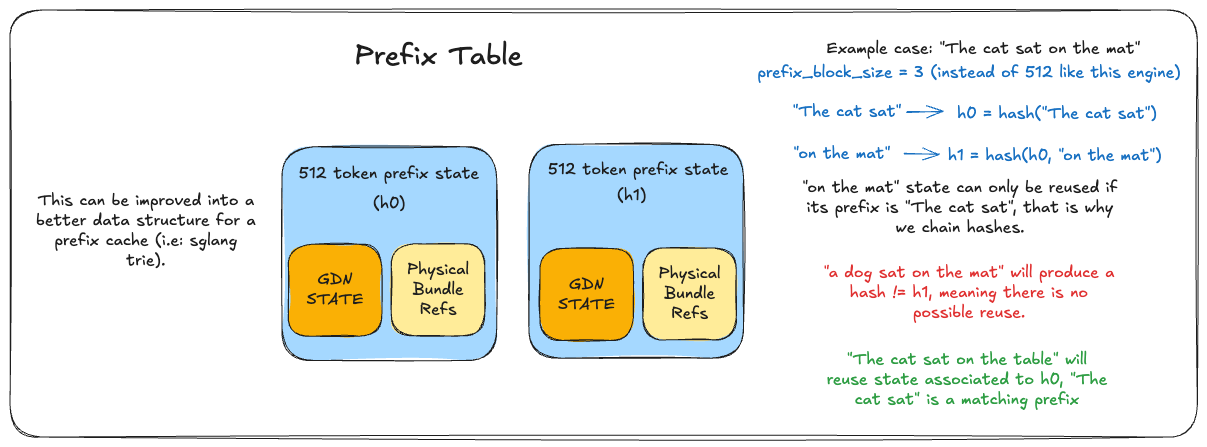
The main design choice is the granularity at which prefixes are cached. Saving entries more frequently improves the hit rate but consumes more memory. Although Qwen 3.8’s linear-attention layers reduce the state required by each sequence, every prefix cache entry still needs about 50 MiB to store the GatedDeltaNet state for all 24 layers (see Appendix B). I currently use a 512-token interval as a reasonable tradeoff, though this value still needs to be tuned using real workload data.

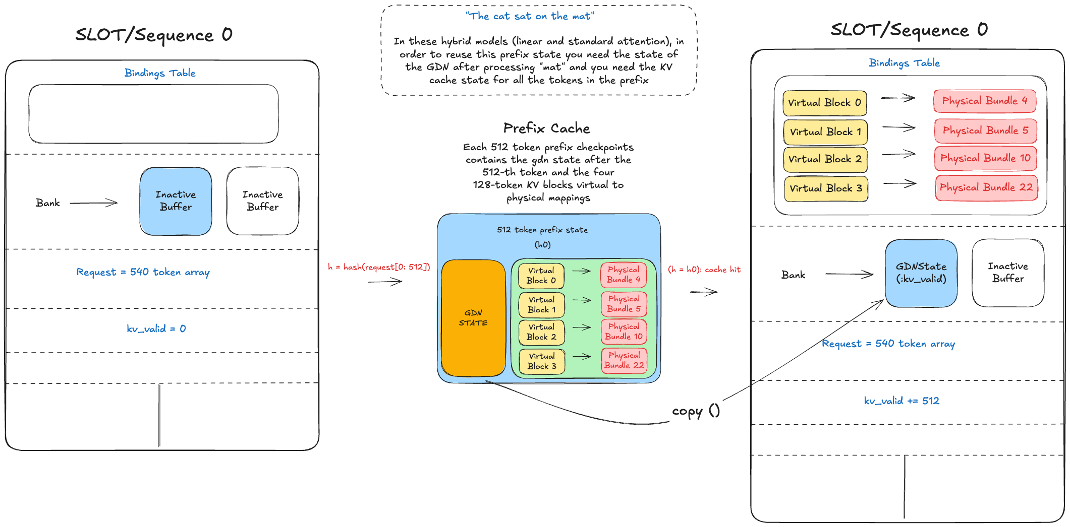
With the prefix cache in place, we can return to what happens when a request enters a slot. The engine hashes the request’s 512 token prefixes and performs a cache lookup. On a hit, it copies the cached GDN state into the slot’s buffer selected by bank, preventing that cache entry from being modified by this new sequence. The corresponding physical KV-cache bindings are then installed in the slot’s bindings table.

The Scheduler Forms a Batch

If we processed each sequence one at a time, we would not get any benefit from supporting concurrent requests. The aggregate speed, meaning the sum of all sequence speeds, would be at most the speed of a single request running in isolation. That is why we want to apply Continuous Batching. It allows us to send tokens from multiple sequences through the model together. The benefit comes from using the weights loaded from memory for more tokens, increasing the arithmetic intensity of the problem.

At this stage, every sequence has a pending = len(request) - kv_valid difference that depends on whether it had a prefix-cache hit. With some caveats (speculative decoding), this difference represents the number of tokens the sequence still needs to send through the model to compute their KV state.

The engine has a fixed capacity for each model pass, which is 128 tokens in MTLQwen. A scheduling policy decides how to divide this capacity between sequences. Sequences with pending = 1 are in the t.g stage and, with speculative decoding enabled, send n_draft tokens through the target model. Sequences with pending > 1 are in the p.p stage, where the scheduler can adjust the size of each processed chunk. Prioritizing p.p favors TTFT, while prioritizing t.g improves throughput and ITL.More p.p capacity lets new requests finish their prompts and reach the first sampled token sooner. More t.g capacity advances live Sequences on each engine step, reducing the delay between tokens and increasing the rate at which output tokens are produced.

From this point on, all tokenization shown in the diagrams is illustrative and does not represent the exact output of Qwen’s tokenizer.

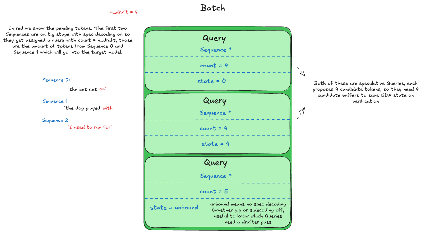
The scheduling policy I chose is simple: every live sequence advances on each step, which is possible because max_slots * n_draft < 128. Each t.g sequence (with spec decoding on) receives a count of n_draft, where count is the number of tokens it will compute. The remaining capacity is then divided equally between the p.p sequences. Each query also has a state property, which stores an offset into the candidates buffer. This buffer preserves the intermediate linear attention states produced while verifying proposed tokens (more on this later).

Sparse K/V Memory Is Reserved

At this point, we know how many tokens each sequence will send through the model, so we can determine how much KV-cache memory it needs. My engine allocates this memory in 128-token blocks. If kv_valid + count crosses a 128-token boundary, the engine requests a new physical block from the OS heap and binds it to the sequence’s virtual address space (see Appendix A: Sparse Buffers).

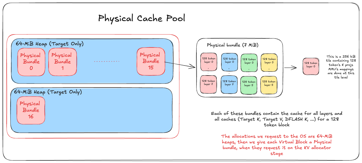
This mapping is also recorded in the bindings table. The engine uses it when publishing a 512-token prefix to the prefix cache and when freeing physical blocks after a sequence ends. The kernels from this engine do not need to read this table, unlike engines such as vLLM. They access virtual memory directly, leaving the virtual-to-physical translation to the MMU.

The Drafter Proposes Tokens

At this point, each sequence has the memory required for its next model pass. Its virtual-to-physical mappings are installed in the MMU and recorded in the sequence metadata, while count identifies how many request tokens it will compute. Each sequence also knows which GDN buffer to read from and write to. If it is using speculative decoding, it additionally knows where to store each verification token’s GDN state in the candidates buffer.

The tokens shown in the DFLASH model diagram are illustrative and do not correspond to the input batch.

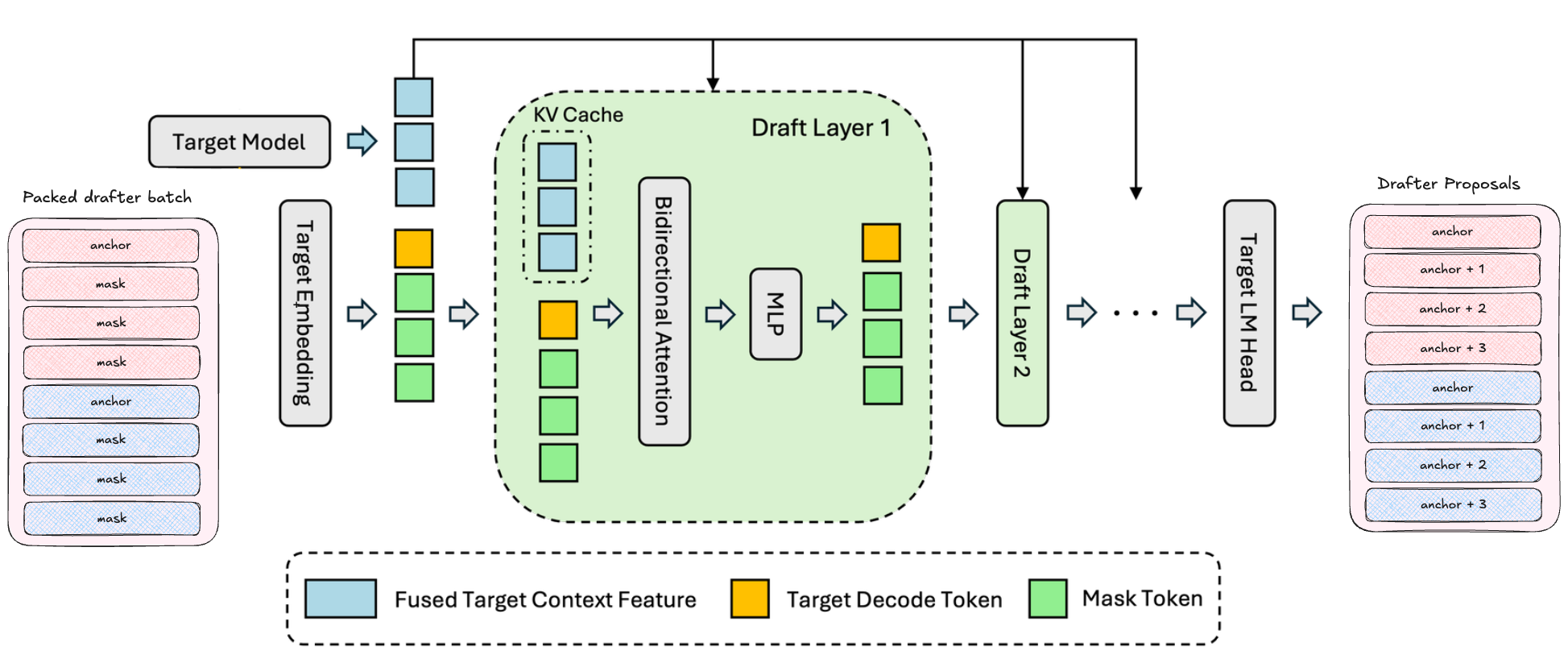
We first build a packed batch containing every Sequence that requires a drafter forward pass, identified by state != unbound (see the Batch building section). Each Sequence follows the drafter’s input format: its anchor token (the last sampled token whose KV has not yet been computed) followed by n_draft mask tokens. The drafter then proposes n_draft tokens for each Sequence. These proposals are later combined with the tokens from those queries with state = unbound (speculative decoding off or p.p stage) to form the target-model batch.

Inputs Are Packed for the GPU

Now that we have the drafter proposals and the remaining target queries, we can pack the input batch and build the metadata the model needs to correctly process these tokens. As shown in this Continuous Batching explanation, the attention kernels must prevent tokens from interacting across Sequence boundaries. For this, we build queryStartLoc, where queryStartLoc[i] gives the starting offset of Sequence i in the packed inputIds. The final entry marks where the packed input ends.

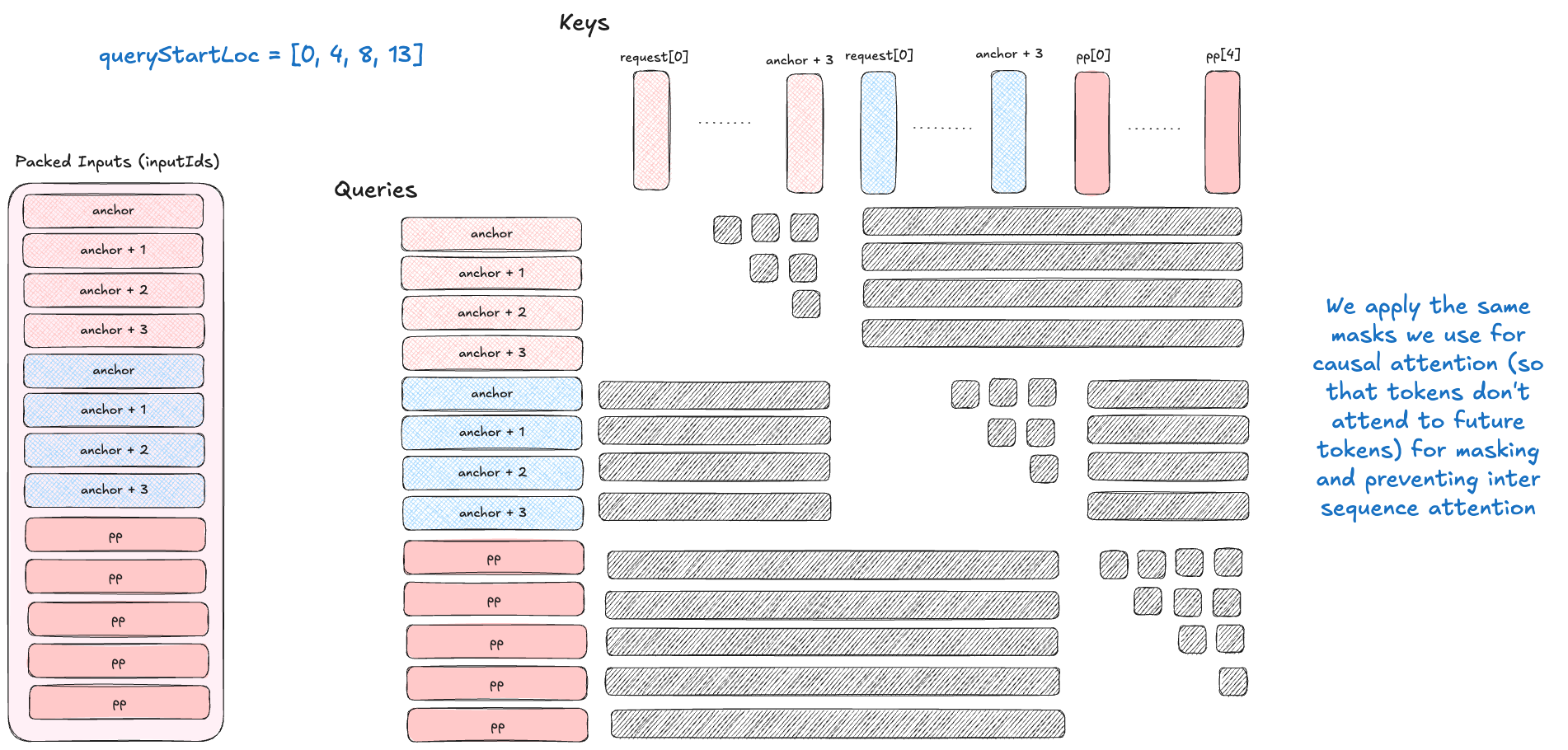
sequenceSlots[i] and batchedKvValid[i] locate each Sequence’s existing KV state. sequenceSlots[i] identifies its slot, while batchedKvValid[i] gives the offset where the new KV computation begins. Everything in [0, kv_valid) has already been computed and is used as attention context.

The Target Model Runs

At this point, the packed inputIds and all the metadata needed to keep each Sequence isolated are ready, so we can run the target model. The kernels need to implement the Qwen 3.8 architecture shown below, as long as their results remain within a reasonable numerical tolerance of a reference Qwen implementation (could be in PyTorch or tinygrad) and they handle the intersequence masking described previously, each part of the architecture can be implemented however we want. This means I can choose how each operation is implemented and which operations are fused together. Since the model runs on a native Metal C++ backend I built, I can profile these kernels through native .gputrace and iterate them until reaching a very good performance level. Most of the performance gains in my engine came from optimizing the quantized linear kernels, which dominate runtime on each forward pass, alongside a decode optimized FlashAttention 2 kernel and a chunked parallel scan that computes the GatedDeltaNet state in 32-token blocks for p.p sequences. More on these kernel optimizations in a future blog.

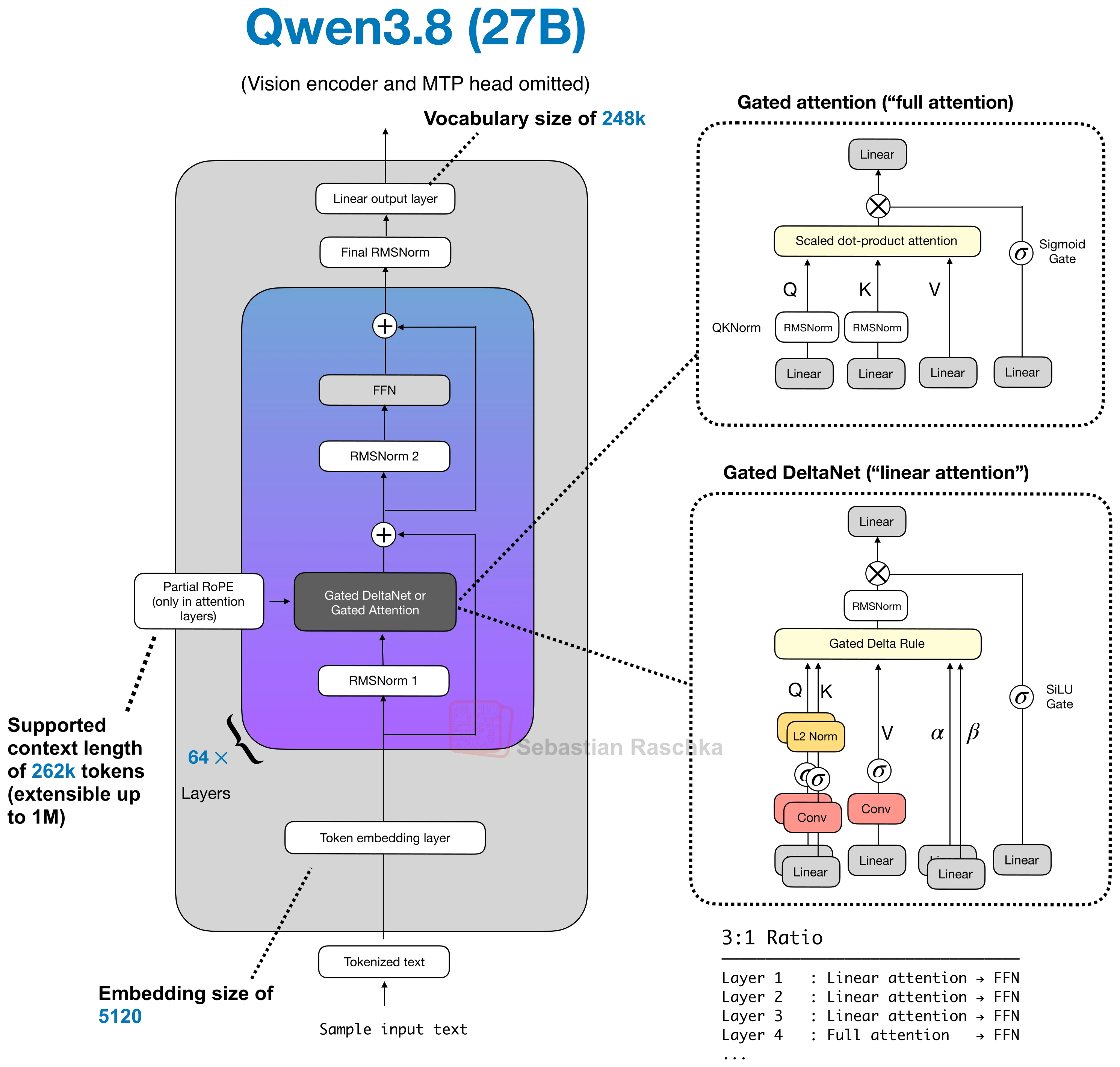
Once the packed batch has run through these kernels, we have the target samples needed to verify the drafter proposals, along with the KV cache and GDN state computed for every Sequence in the batch.

State is injected to the drafter

As shown in the packed DFlash pass, the drafter relies on context produced by the target model. During each target pass, besides updating the target KV cache and sampling where required, we encode this context into the drafter’s cache.

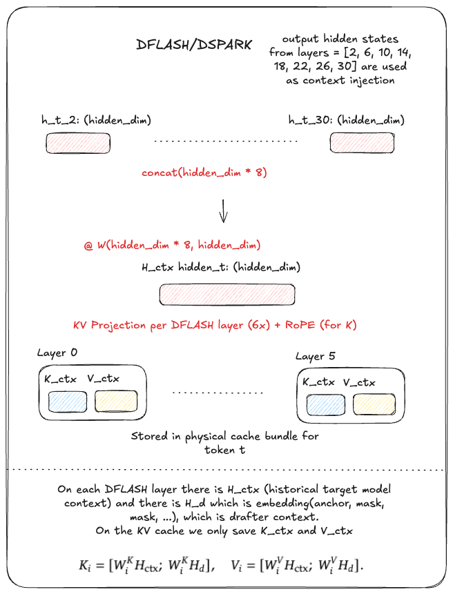
For every processed token $t$, we capture the target hidden states after layers 2, 6, 10, 14, 18, 22, 26, and 30. These are concatenated and projected down to the drafter’s hidden dimension, producing the context representation $H_{\text{ctx},t}$.

Each of DFlash’s six attention layers projects $H_{\text{ctx},t}$ into its own $K_{\text{ctx}},V_{\text{ctx}}$. These are stored in the same physical cache bundles as the target KV and addressed by (sequence slot, token position) (see Appendix A). During drafting, the cached context K/V is attended together with the temporary K/V produced by the packed anchor and mask tokens.

Tokens and State Are Committed

For Sequences using speculative decoding, we first compare each drafter proposal with the corresponding target sample. My engine uses greedy decoding, so a proposal is accepted only when both tokens are equal. Sampling-based verification instead draws u ~ U(0,1) and accepts with probability min(1, p_k / q_k). This can accept proposals based on probability overlap rather than exact equality, but requires retaining vocab_size probability distributions for each proposed token until verification and resampling ends. I still need to evaluate whether the higher acceptance rate is worth this memory cost. We then commit the accepted prefix by advancing kv_valid by the number of accepted tokens. With greedy decoding, the target sample at the first mismatch becomes the new anchor and is appended to request for the next forward pass.

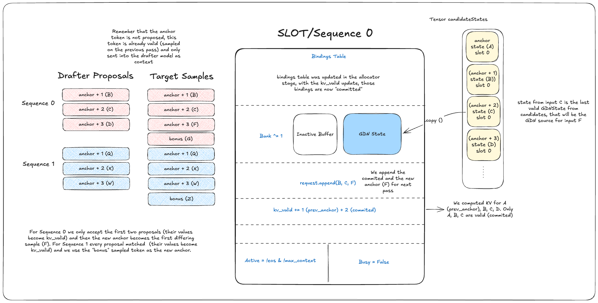
This is where the purpose of the candidateStates buffer mentioned in the Batch Building section becomes clear. In linear-attention models, the memory is a fixed-size matrix updated in place as tokens pass through the model. If we wrote the final state directly into the slot and then rejected the last proposal, that state would still include an unaccepted token. In the figure, rejecting D would leave us with an invalid state. Instead, we save the state after each proposal in candidateStates, then copy only the state after the last accepted proposal into the slot’s GDN buffer selected by bank. If C is the last accepted proposal, we commit the state produced after C.

Tokens from p.p queries and t.g queries with speculative decoding disabled advance without verification. For a p.p Sequence, every token processed in this pass is already part of request, so kv_valid advances by count. For a non-speculative t.g Sequence, the previous anchor now has its KV computed, so kv_valid advances by one and the target sample is appended to request as the new anchor.

Every Sequence that crosses a 512-token boundary then extends its prefix hash with the newly completed 512-token chunk and publishes an entry to the prefix cache. This entry contains the GDN state after the final token in that prefix, together with all the KV-cache bindings needed to restore it in another slot.

At this point, one engine step is complete. The engine can accept new requests into available slots and send the remaining live Sequences back through the loop until the request ends.

Design Tradeoffs and Current Limitations

• The current 512-token prefix granularity gets few hits because the prefixes are too long. Shorter intervals would improve the hit rate but make memory usage explode. One possible solution is to publish shorter prefixes only up to request[max_prefix], where the data says reuse is more likely.

• The engine currently supports Qwen 3.8 and 3.5, which share the same architecture. Supporting more models should be straightforward, with new kernels required only when an architecture introduces different operations, such as Kimi’s linear attention or DeepSeek’s MLA. Sliding-window attention is probably the next addition, since more models are adopting it.

• I still need to tune the current 128-token block size. Smaller blocks waste less memory when partially filled but require more frequent allocations, while larger blocks reduce allocation overhead at the cost of more unused memory.

• Currently, the C++ runtime compiles the Metal kernels and builds their pipeline states when the model is loaded. I could instead precompile the kernels into a .metallib and use a binary archive to reduce the remaining pipeline compilation at startup. However, at my current development stage, where I am constantly iterating on the kernels, runtime compilation is the best option.

Appendix A: Sparse Buffers

There is a very good blog post explaining how sparse buffers work and why they are useful for KV caches. In short, sparse buffers allow us to reserve a large contiguous virtual address range for every slot in our engine, enough to hold the KV cache for maxContext = 65k tokens without committing that amount of physical memory upfront (like llama.cpp does).

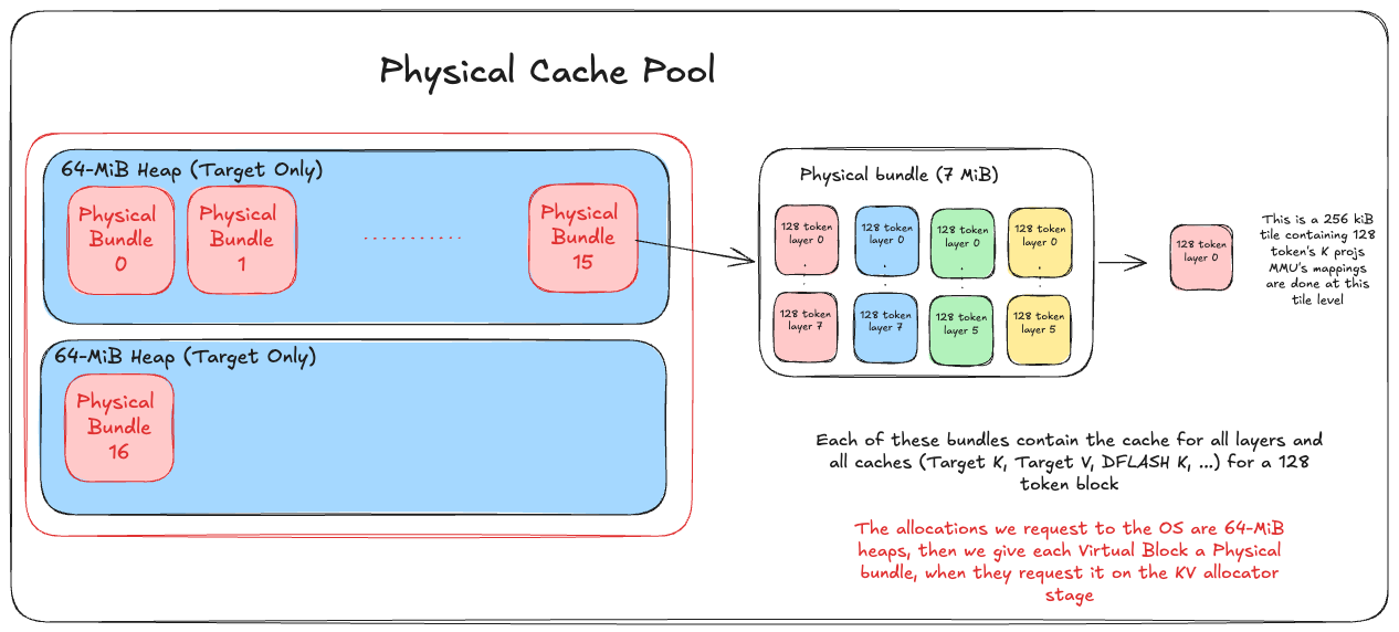
In my engine, the KV cache is managed in 128-token logical blocks. To simplify allocation and addressing, all cache tiles for one block across every layer and cache type (Target K, Target V, DFlash K, and DFlash V) are allocated as a single physical bundle. Each tile is a 256 KiB page holding 128 tokens for one (cache, layer) pair, so with DFlash enabled, a bundle contains 28 tiles and occupies 7 MiB. As with virtual memory in an operating system, these bundles do not need to follow the logical ordering in physical memory. Before each forward pass, we find which logical blocks the batch will touch and allocate any missing bundles from the shared placement heap pool (see the cache pool figure). Their tiles are then mapped into the corresponding sparse K/V buffers. Metal records these mappings in the GPU page tables, and the MMU handles the translation, keeping tokens contiguous within each virtual K/V layer region even when their physical backing is not.

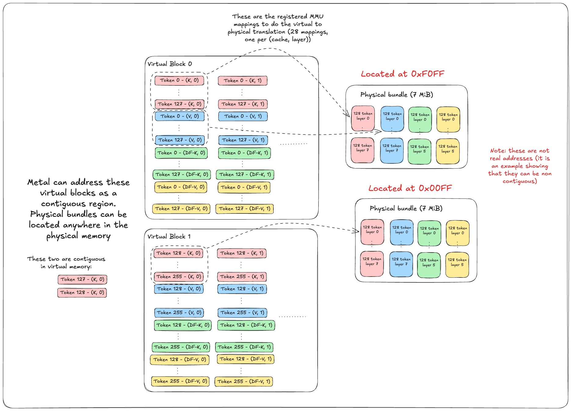
All slots allocate from the same physical pool. When a Sequence is destroyed, its mappings are removed and any unreferenced bundles return to the pool. When reusing a cached prefix, the same physical bundles can also be mapped into the virtual blocks of multiple slots. In addition, each bundle has a ref_cnt, similar to vLLM, which tracks how many mappings reference it and whether it can be evicted when memory is limited.

Appendix B: Standar Attention vs GDN State

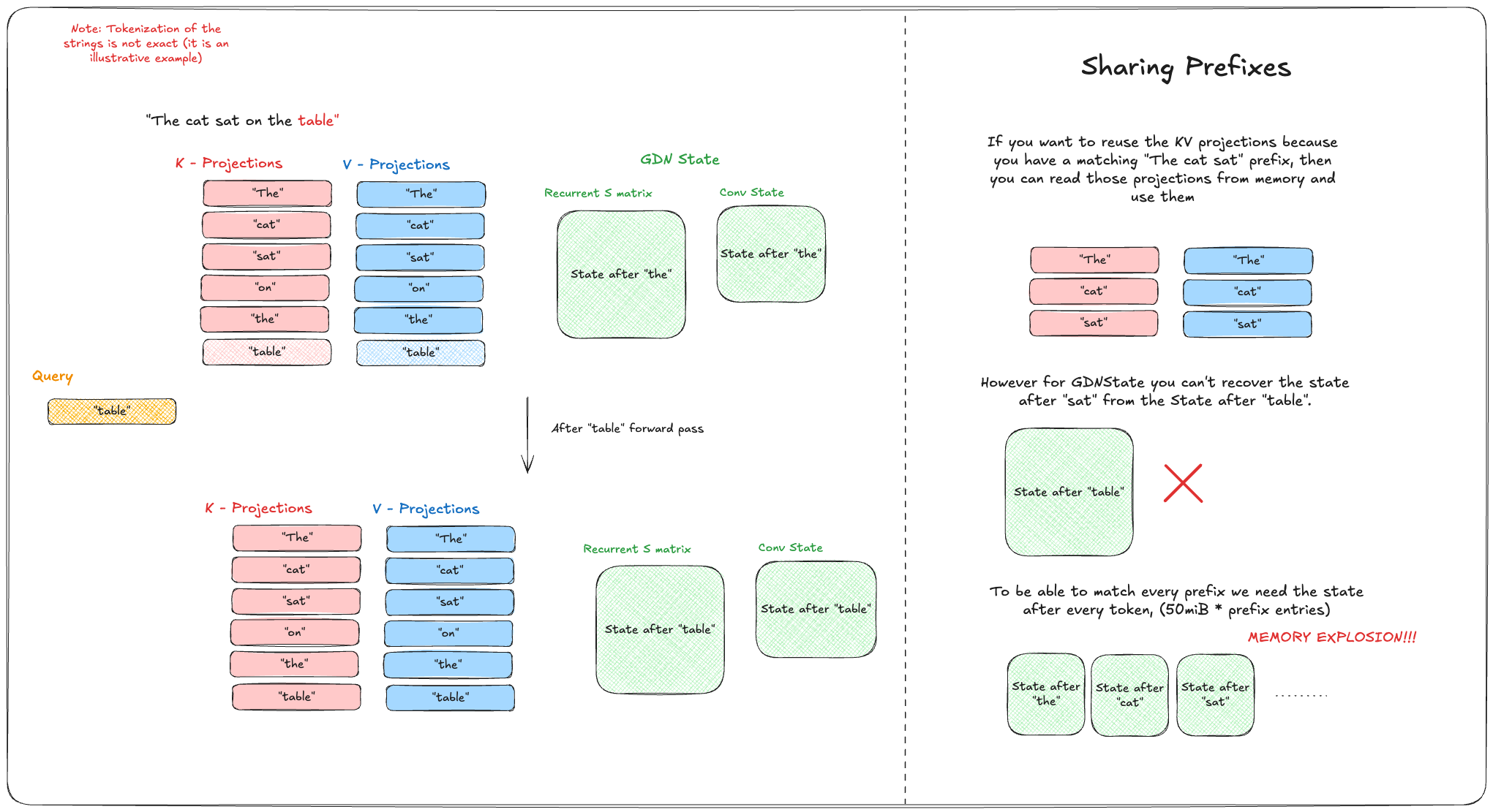
In standard causal attention, the query for “table” attends to the K and V projections of every token up to and including itself. Its own projections are then appended to the KV cache for subsequent tokens. The cache grows linearly with sequence length.

GatedDeltaNet instead compresses the entire prefix “memory” into a fixed size recurrent matrix and a small convolution state (50 MiB for Qwen 3.5). Both are updated after every token, so the memory required to maintain one Sequence remains constant as its context grows. This is the main advantage linear attention brings to the table.

This compression makes sharing prefixes more complicated. With a KV cache, the K/V projections are stored per token, so if two requests share the first $n$ tokens, we can reuse the cache up to that point. A GDN state represents one exact prefix and cannot be rolled back to an earlier one. Supporting $P$ prefix boundaries therefore means either storing $P$ full GDN state snapshots, which removes its memory advantage, or recomputing from an earlier checkpoint, which removes much of the speedup from prefix caching. One final difference is that KV-cache reuse can point multiple Sequences to the same physical blocks because those blocks remain read-only. GDN state is overwritten as a Sequence advances, so each cached state needs dedicated prefix-cache memory and must be copied into the slot when reused.

The tradeoff I adopted for this engine is to cache prefixes at a much coarser granularity than other engines, using 512 token boundaries. This keeps prefix-cache memory usage manageable while still allowing hits on long shared prefixes, such as system prompts and tool definitions.

---

1. The engine was originally built for Qwen 3.5, but Qwen 3.8 has the exact same architecture, so it works natively with it.
2. The quantization type determines how the weights are packed and dequantized, while the shape determines the tiling and dispatch configuration that works best with it (maximizing occupation).
3. A ComputeCommandEncoder records which PipelineState (an executable kernel) to run, the resource bindings for the buffers it touches, and the dispatch dimensions. Encoders are stored inside a CommandBuffer, which I mostly treat as their submission wrapper, and that buffer is then committed to the GPU CommandQueue. Every GPU operation, including rendering and compute kernels, is ultimately submitted through this CommandQueue.
4. More p.p capacity lets new requests finish their prompts and reach the first sampled token sooner. More t.g capacity advances live Sequences on each engine step, reducing the delay between tokens and increasing the rate at which output tokens are produced.
5. From this point on, all tokenization shown in the diagrams is illustrative and does not represent the exact output of Qwen’s tokenizer.
6. The tokens shown in the DFLASH model diagram are illustrative and do not correspond to the input batch.
7. Most of the performance gains in my engine came from optimizing the quantized linear kernels, which dominate runtime on each forward pass, alongside a decode optimized FlashAttention 2 kernel and a chunked parallel scan that computes the GatedDeltaNet state in 32-token blocks for p.p sequences. More on these kernel optimizations in a future blog.
8. I still need to evaluate whether the higher acceptance rate is worth this memory cost.